Avocado Prices
Inflation has captured the nation’s attention this year. So when I read about a problem of how to measure price elasticity, my interest perked. I searched Kaggle and found a price, demand dataset about avocados. There is no substitute for avocado toast. Shopping at the supermarket, I buy more avocados when prices are low, but consistently buy avocados to enjoy the sweet breakfast toast. Let’s use data to prove my intuition.
Price Elasticity
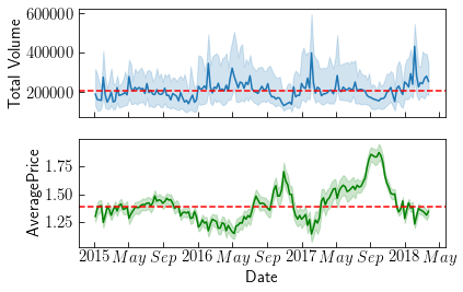
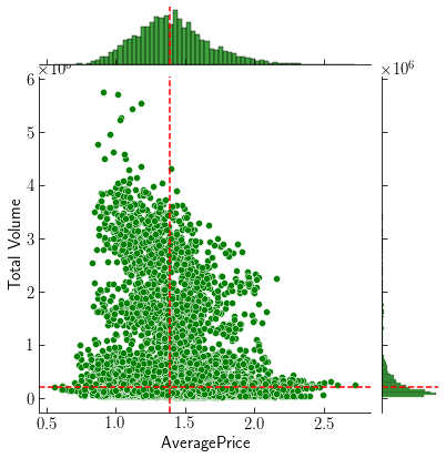
Comparing Prices to Demand shows the Median Price: $1.39 and Median Demand 205K. Observations are collected over 169 days in 53 regions. Over time, prices negatively correlate with demand. Higher prices in September correlate with less Volume over the same season. Lower prices below median correlate with higher demand. Prices are generally similar across all regions and time. Regions differ considerably in value because of their sizes, but the distribution appears consistent within a 95% confidence interval.
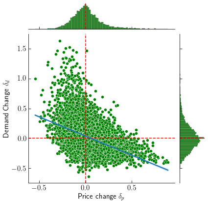
A simple economic description is to compare the change in price $\delta_p$ to change in demand $\delta_d$. They are related by \(\delta_d = E \delta_p\) where $E$ is the elasticity of a good. Elasticity is always negative, with $-1$ meaning demand changes exactly with prices, and being considered inelastic if $0$. Inelastic goods such as air and water are necessary for functioning human.
Elasticity follows the basic idea of supply and demand: lower prices should increase demand, and higher prices should decrease demand. However, if the good is indespensible (avocado toast?) demand would be inelastic to changes in prices. Computing a linear regression gives the avocado elasticity of $-.64$. Analyzing the scatter plot shows the regression is consistent for high prices, although when prices drop there is a high likelihood demand could skyrocket.
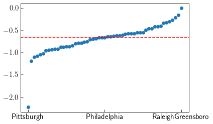
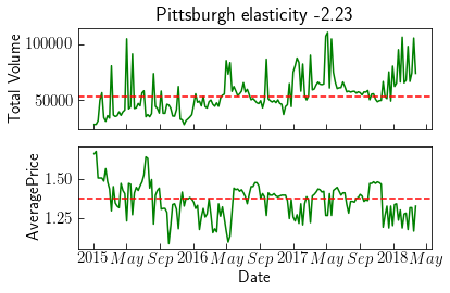
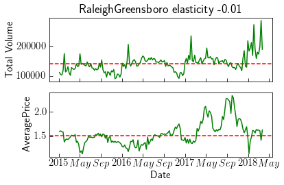
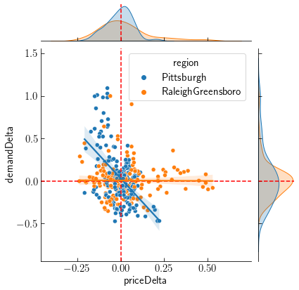
Regressing within each region shows elasticity varies $-.69 \pm 0.33$ on average. Outliers on either end of the scale are Pittsburgh $E=-2.23$ which is very elastic, and RaleighGreensboro $E=-0.01$. Viewing the time series is not very intuitive. Pittsburgh is a smaller market than Raleigh and avocado prices are much more variable. Comparing the price and demand changes shows Pittsburgh demand is not sensitive to price changes, whereas Raleigh exhibits a clear correlation.
Conclusion and Future Work
Widespread inflation has soured sentiment this year because there are few alternatives for price increases. Understanding how elasticity works sheds light on why the current situation is frightening. Gasoline price increases do not dent demand very much, so it is an inelastic good. If consumers have no choice but to pay higher prices for the same amount of demand, then the real value of their purchases will inevitably fall.
A more thorough analysis would compare many goods at once. If the price of one good, say oat milk, increases, then a viable substitute would be dairy creamer. The price increase in one good is offset by increased demand for its substitute. The same linear regression model can estimate this larger problem, stated as
\[\Delta_d = \Delta_p E^d\]where $\Delta_{d,p}$ are a $N \times n$ matrices of $n$ goods measured over $N$ days, and $E^d$ is a $n \times n$ demand elasticity matrix. Suppose $E^d_{11}=-0.4$ and $E^d_{21}=0.2$. This means a $1\%$ price increase of the first good, with other prices kept the same, causes demand for the first good to drop $0.4\%$, and demand for the second good increases by $0.2\%$. In this case the second good is a partial substitute for the first good.