Sine Fitting
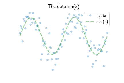
Sine signals are not lines. So how does a linear model fit a sine curve? We examine this problem by observing $N = 100$ datapoints along 2 periods of a sine curve. The data comes from sampling $y = \sin(x) + \epsilon$, where $\epsilon$ is some noise. The figure above shows the $N=100$ datapoints as blue dots and the underlying green sine curve.
A line between two points
Straight lines are be defined by two numbers, slope $m$ and intercept $b$. Given some input $x$, the output is
\[y = mx + b.\]The two unknowns $b, m$ can be solved directly with two training pairs $x_1, y_1$ and $x_2, y_2$ and some linear algebra. Begin with a system of equations
\[\begin{bmatrix} y_1 \\ y_2 \end{bmatrix} = \begin{bmatrix} 1 & x_1 \\ 1 & x_2 \end{bmatrix} \begin{bmatrix} b \\ m \end{bmatrix}\]and then row reduce to get the pivots
\[\left[ \begin{array}{cc|c} 1 & 0 & y_1 - x_1 \frac{y_2 - y_1}{x_2 - x_1} \\ 0 & 1 & \frac{y_2 - y_1}{x_2 - x_1} \\ \end{array} \right].\]The second row is the slope $m=\frac{y_2 - y_1}{x_2 - x_1}$. Take the difference in heights $y_2-y_1$, and normalize by the range $x_2 - x_1$. The intercept is found by back substitution $b = y_1 - x_1 m$. The figure above shows choosing two random data points and the slope and intercept between them.
Which pair of data generates a line with the best fit? Given $N=100$ data points, a brute force approach enumerates all combinations of pairs ${100 \choose 2} = 4950$, fits the slope and intercept to each, and computes a residual score, also called the loss function. A common loss is to take the difference between the actual value $y$ and predicted value $\hat y = mx + b$, square the difference so it’s positive, and take the average
\[\text{Mean Square Error (MSE)} = \frac{1}{N} \sum_{i=1}^N (\hat y - y_i)^2.\]Another loss function uses the absolute difference between predicted and observed values
\[\text{Mean Absolute Error (MAE)} = \frac{1}{N} \sum_{i=1}^N |\hat y - y_i|.\]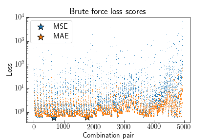
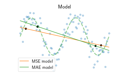
Plotting the (MSE, MAE) loss for each combination shows the MSE produces higher scores for bad fits than MAE. Pairs of data that are close to each other $x_1 - x_2 \approx 0$ enable large slopes which quickly diverge from the actual values and yield large losses. Points further away from each other average out this effect. Different loss functions yield different optimal models. MSE tends to minimize large differences, i.e., outliers, while MAE likes to cluster around groups of points and ignore outliers. In this sine dataset, both models choose points at the opposite ends of the range. As expected, MSE tries to average all the points, while MAE tends towards the groups of points at the top-left and bottom right.
Least Residual fit
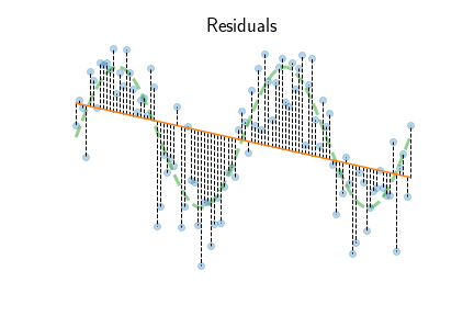
Instead of enumerating over all possible datapoints to find the best line, let’s find the best model by examining the all residuals
\[r^{(i)} = \hat y^{(i)} - y^{(i)}\]for each data point $i = 1, \ldots, N$. Residuals measure how well the model $\hat y^{(i)} = b + m x^{(i)}$, with certain slope $m$ and intercept $b$ parameters, fits the observed data $y^{(i)}$. A relative prediction error measure uses root mean square ratio $\textbf{rms}(r^d) / \textbf{rms}(y^d)$. The MSE and MAE models above produce $93\%$ and $95\%$ relative prediction error because the linear model cannot capture the sine curve.
An objective to find the best model parameters $\theta = (m, b)$ would be to minimize the total length of all residuals
\[\text{minimize } \|r^d\| = \| \hat y^d - y^d \|\]where $\| \cdot \|$ denotes the norm, or length, of a vector. A common norm is the euclidean norm
\[\| r \|_2 = \sqrt{r_1^2 + r_2^2 + \cdots + r_N^2}\]basically Pythagoras in $N$-dimensional space. Another type of norm uses the absolute value
\[\| r \|_1 = |r_1| + |r_2| + \cdots + |r_N|.\]Note that $\text{MSE} = (1/N) \|r\|_2^2$ and $\text{MAE} = (1/N) \|r\|_1$.
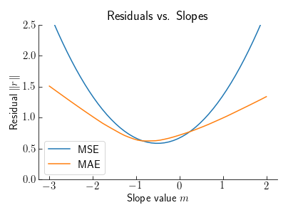
The figure above shows the residual MSE and MAE as a function of line slope $m$. What’s interesting is both the square and absolute error have a unique optimal slope $m^*$. As shown in the previous section, the MSE slope tends to be closer to the average, while MAE adjusts to be closer to groups of points. MSE also achieves a smaller error than MAE, because $r_i^2 < |r_i| < 1$.
Using the eucidean norm of the residuals, we can solve exactly for the best model $\hat \theta$. First represent the system of equations
\[\begin{bmatrix} y_1 \\ y_2 \\ \vdots \\ y_N \end{bmatrix} = \begin{bmatrix} 1 & x_1 \\ 1 & x_2 \\ \vdots & \vdots \\ 1 & x_N \end{bmatrix} \begin{bmatrix} b \\ m \end{bmatrix}\]in matrix format
\[y^d = A \theta.\]The notation expresses $N$ measurements in the $N$-vector $y^d$, expressed in the 2 basis $N$-vectors $2N$ numbers into the matrix $A$ which is skinny, i.e., it is taller than it is wide. The vector $\theta = (b, m)$ represents the model parameters that we want to find. Row reducing and finding each parameter via backsubstitution will not work because there are too many equations and not enough variables. Unless every datapoint is a copy of another, the equations have no solution. Instead of an exact solution, we seek the best model $\hat y^d = A \hat \theta$ that fits the data.
Finding the optimal $\hat \theta$ that minimizes the euclidean residual can be shown to have the formula
\[\hat \theta = (A^T A)^{-1} A^T y^d\]known as the Least-Squares solution. Performing the algebra to find the slope gives the equation
\[m = \frac{\mathbf{std}(y^d)}{\mathbf{std}(x^d)} \rho\]where $\rho$ is the correlation coefficient. Correlation is best understood by examining the demeaned data
\[\begin{align*} \tilde{x}^d &= x^d - \mathbf{avg}(x^d) \mathbf{1}\\ \tilde{y}^d &= y^d - \mathbf{avg}(y^d) \mathbf{1}\\ \rho &= \frac{(\tilde{x}^{d})^\textsf{T} y^d}{\| \tilde{x}^d \| \| \tilde{y}^d \|}. \end{align*}\]Correlation measures similarity between two vectors in $N$ dimensional space (more precisely the cosine angle $\cos \angle(x, y)$). If every element of $\tilde{x}^d$ and $\tilde{y}^d$ are the same, then the numerator and denominator have the same value so $\rho = 1$. Conversely if they have the same magnitude but opposite sign, then $\rho = -1$. In between, corresponding values are different, and the correlation decreases. For the sine curve $\rho = -0.36$ and the slope $m=-0.51$.
Solving for the intercept uses substitution
\[b = \textbf{avg}(y^d) - m \; \textbf{avg}(x^d)\]and putting the model together gives the formula
\[\hat y = \textbf{avg}(y^d) + \rho \frac{\mathbf{std}(y^d)}{\mathbf{std}(x^d)} (x - \textbf{avg}(x^d))\]and rearranging provides a useful insight
\[\frac{\hat y - \textbf{avg}(y^d)}{\textbf{std}(y^d)} = \rho \frac{x - \textbf{avg}(x^d)}{\textbf{std}(x^d)}.\]The left side is the normalized predicted output. The right side is the normalized change in input, with $\rho$ as a shrinking factor. If $\rho \approx 1$, then changes in $x$ are nearly one-to-one as changes in $\hat y$. But as correlation decreases, then changes in $x$ do not modify the response as much. The predictions regress to the mean. If $x$ is uncorrelated with $y$, the best prediction is the mean $\textbf{avg}(y^d)$.
Fitting a Nonlinear Function with a Linear Model
Polynomial curves can be written as a linear model. For example, a quartic curve
\[y = a_0 + a_1 x + a_2 x^2 + a_3 x^3 + a_4 x^4\]can be written as a basis form
\[\begin{bmatrix} y_1 \\ y_2 \\ \vdots \\ y_N \end{bmatrix} = \begin{bmatrix} 1 & x_1 & x_1^2 & x_1^3 & x_1^4 \\ 1 & x_2 & x_2^2 & x_2^3 & x_2^4 \\ \vdots & \vdots& \vdots& \vdots \\ 1 & x_N & x_N^2 & x_N^3 & x_N^4 \end{bmatrix} \begin{bmatrix} a_0 \\ a_1 \\ a_2 \\ a_3 \\ a_4 \end{bmatrix}.\]Now we have $N$-quartic equations which use the same model $\theta = \begin{pmatrix} a_0 & a_1 & a_2 & a_3 & a_4 \end{pmatrix}$. The least-squares objective is to find the set of coefficients which best approximate the dataset. Any polynomial of degree $p$ can be represented this way.
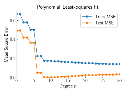
Fitting higher and higher polynomials will always reduce the error compared to the dataset $y^d$. Comparing the training residual MSE to the residual of the actual $\sin(x)$ curve shows higher degrees result in smaller training error. The animation shows above the optimal value $p=8$ the predictions capture variation produced by the noise.
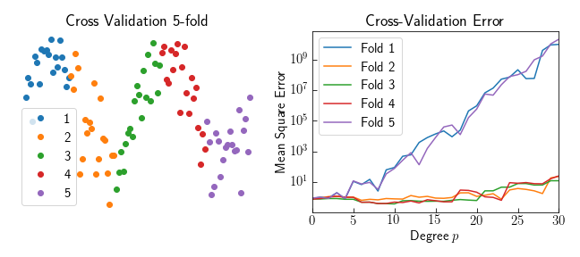
Without knowledge of the underlying model we can approximate a validation error by excluding part of the dataset from the fitting procedure. Leaving out part of the dataset, and fitting a model to the rest is called cross validation. Using 5-folds, one fifth of the data is left out while the rest is used to fit the model. The validation error would take the RMS value of all the left out folds. Using this technique on a polynomial fit shows a shortcomming of this type of model: polynomials should never extrapolate beyond the dataset. Folds 1 and 5 leave out the tails of the dataset, and the validation error quickly grows for degrees greater than 4.
Regularization
The basis idea can be extended for any function that is linear in its coefficients. Consider a sum of sines and cosines
\[f(x) = \sum_{k=1}^K \alpha_k \cos(\omega_k x) + \beta_k \sin(\omega_k x)\]where $\omega_k = k \omega_1$ is a integer multiple of some fundamental frequency. The basis $A$ has $2K$ parameters to estimate: the amplitude of each cosine and sine for each frequency $k\omega_1$. A least squares fit will accurately model the dataset, however the cosine coefficients are on the order of $\alpha_k \approx 10^{12}$. We can use knowledge that the coefficients should be small (the exact model with $\omega_1 = \pi /2$ is $\beta_4 = 1$). In order to penalize large coefficients, we augment the least squares objective
\[\text{minimize} \quad \| A \theta - y^d \|_2 + \lambda \| \theta \|_2\]with a new tuning parameter $\lambda$. This is called Ridge Regression.
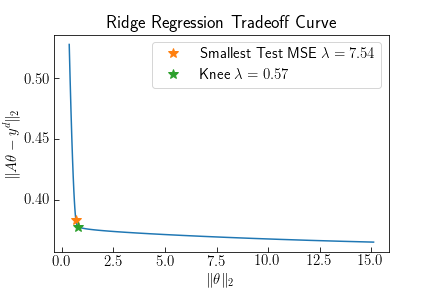
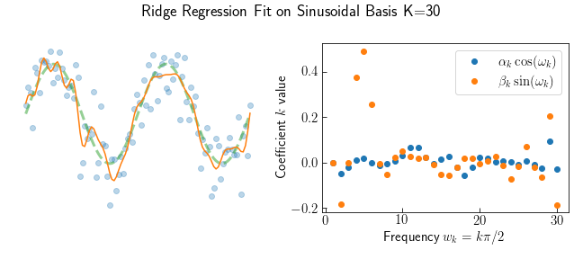
Sweeping through $\lambda = [0.001, 100]$ traces out a tradeoff curve between the coefficient size and residuals. The curve has an obvious knee, where increasing $\theta$ does not return much smaller residuals. Comparing the knee to the smallest Test MSE of the actual sine curve shows this is a good hueristic for choosing the best $\lambda^*$. The plot below shows the model prediction using the knee-optimal regularization, and the coefficient values. The largest coefficients are $\beta_4, \beta_5, \beta_6$. Some higher frequencies are present which try to fit the noise.
Ridge regression tries fitting the noise in the data and the model excites many frequencies. Attempting to choose the fewest number of frequencies (called the cardinality $\textbf{card}(\theta)$) is a NP-hard combinatorial optimization problem with $K! / (k! (K - k)!)$ possibilities. Each $k$ subset of frequencies requires enumerating over all possible models with nonzero coefficients. With $K=30$ there are over 1 Billion models to check.
Fortunately this problem can be solved in polynomial time using a different regularization technique
\[\text{minimize} \quad \| A \theta - y^d \|_2 + \lambda \| \theta \|_1\]by minimizing the absolute value of the coefficients. This is called the Lasso selector. This is no longer Least-Squares and there is no formula which directly solves the minimization. Instead an iterative algorithm traverses the parameter space to find a global minimum. Discussing how this works is the subject for another post, so I use a library function sklearn.linear_model.LassoCV. This takes a sequence of $\lambda$ and returns the best model fit by 5-fold cross-validation.
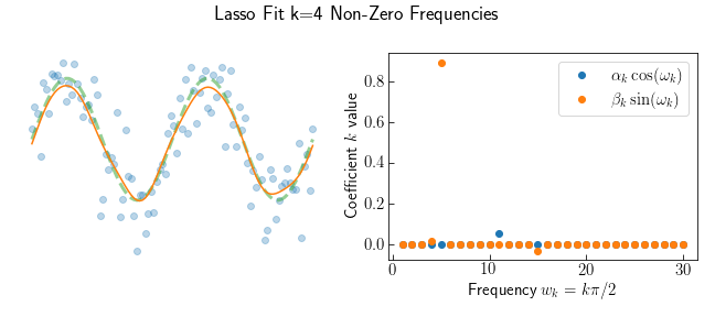
Lasso finds the best model has 4 non-zero frequencies and the most significant is $\beta_5$. Comapared to Ridge Regression the Lasso fit is much closer to underlying sine curve.
Conclusion
A sinusoid is a highly nonlinear function. Fitting a line $y=b + mx$ is an obviously terrible model, but illustrative for how a model fitting procedure should work. A guess and check procedure requires many checks and becomes infeasible for large datasets. Least-Squares incorporates finds an optimal line fit by correlating the variance in $x$ with variance with $y$. Transforming $x$ into a different basis enables a general linear model fit, such as with polynomials or sinusoids. Regularizing the model coefficients restricts the large basis space to reasonable values.